Documentation & User Guide
Welcome to the official documentation for DataSynth Pro. This comprehensive manual provides detailed guidance on configuring parameters for various statistical modules to synthesize robust, academically viable, and statistically valid datasets completely offline.
1. Generating Multiple Indicators Simultaneously
1.1 Prerequisites & Launching
Double-click the executable file to launch the application.
Security Notice: If your antivirus software flags the executable as a false positive, please add it to your local exclusion or whitelist to ensure uninterrupted operation.
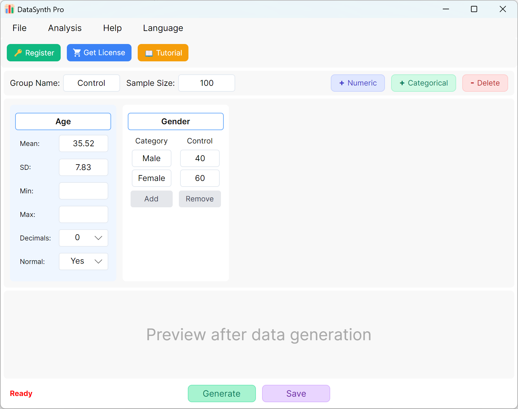
Figure 1.1: User Interface / Operations (Main Interface)
1.2 Parameter Configuration
By default, the application pre-populates two continuous variables, 'Age' and 'Gender', to serve as quick references. The group designation defaults to 'Control Group', and the sample size is set to '100' cases. If your study requires multiple groups, you can generate and export each group's dataset sequentially by updating the parameters for each run.
- Adding Continuous Numerical Variables: To add a new quantitative variable, click the + Numeric button. You can then specify the Indicator Name (e.g., 'Body Mass Index' or 'BMI'), Mean, Standard Deviation, and Decimal Places. The Minimum and Maximum boundary fields are optional and can be left blank if you do not have specific value limitations.
- Data Distribution Settings: By default, generated numerical metrics follow a normal distribution. If you require non-normally distributed data, simply set the Normal Distribution option to No.
Distribution Tuning: A normal distribution relies on a natural variance range; restricting the Minimum and Maximum boundaries too tightly will truncate the normal curve and may result in non-normally distributed values. If this occurs, try widening the boundaries or removing the Min/Max limits entirely.
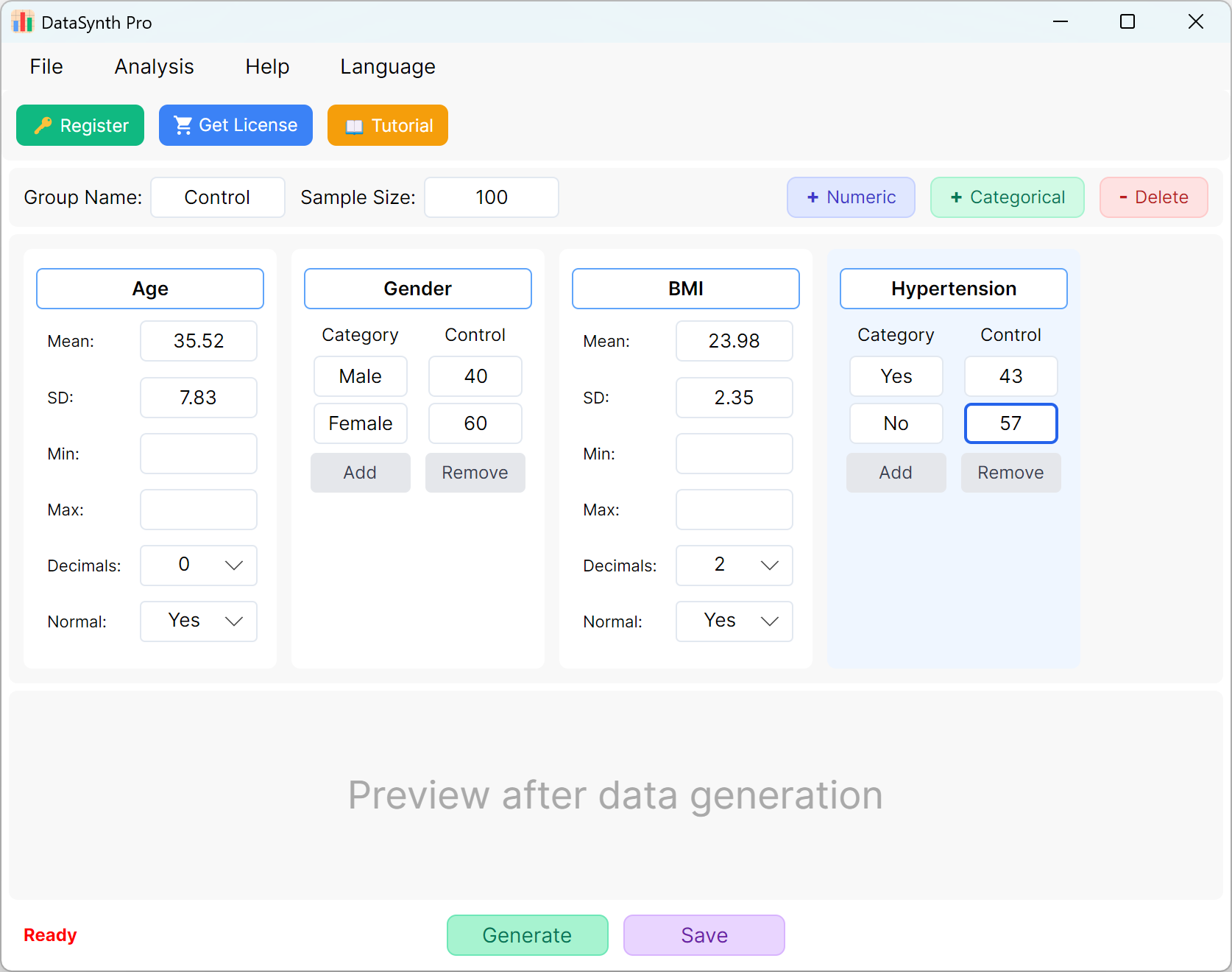
Figure 1.2: User Interface / Operations for Adding Variables
1.3 Adding Categorical Variables
Click the + Categorical button to continue adding qualitative variables (e.g., 'Hypertension'). You can input category names and their corresponding target distributions or proportions. The sum of the categorical proportions will be scaled dynamically to match your configured sample size.
1.4 Executing Generation
Click the Generate button to synthesize the requested number of records. Once calculated, a descriptive statistics summary window will pop up, enabling you to verify whether the actual generated values align with your configured parameters.
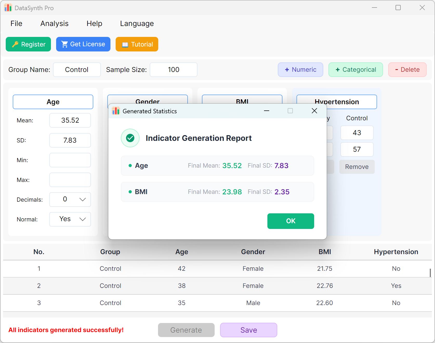
Figure 1.3: User Interface / Operations for Executing Generation
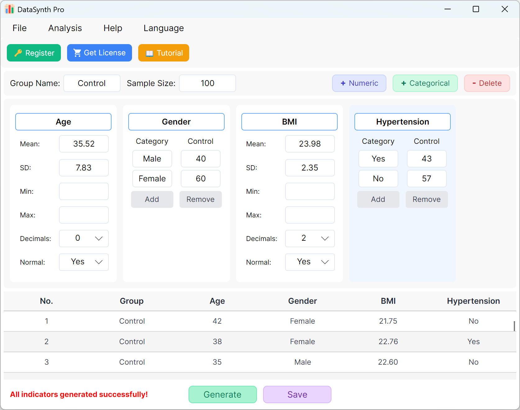
Figure 1.4: User Interface / Operations for Displaying Data
1.5 Exporting and Verifying
Click the Save button to export the generated dataset as a standard Excel file. If you open the exported spreadsheet and calculate the descriptive statistics for 'Age' (rounded to two decimal places) using standard Excel formulas, the actual mean and standard deviation will perfectly match your initial settings.
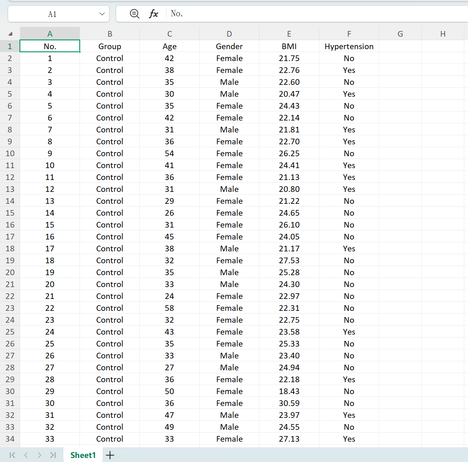
Figure 1.5: Exporting Generated Tables to Excel
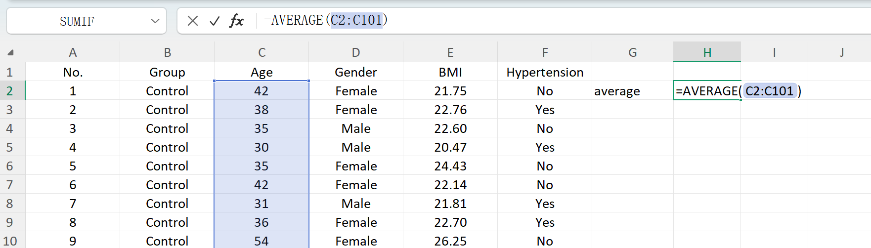
Figure 1.6: Excel Operations for Calculating Mean
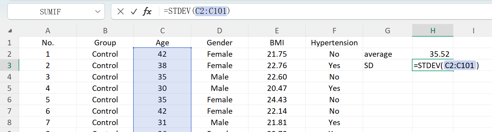
Figure 1.7: Excel Operations for Calculating Standard Deviation
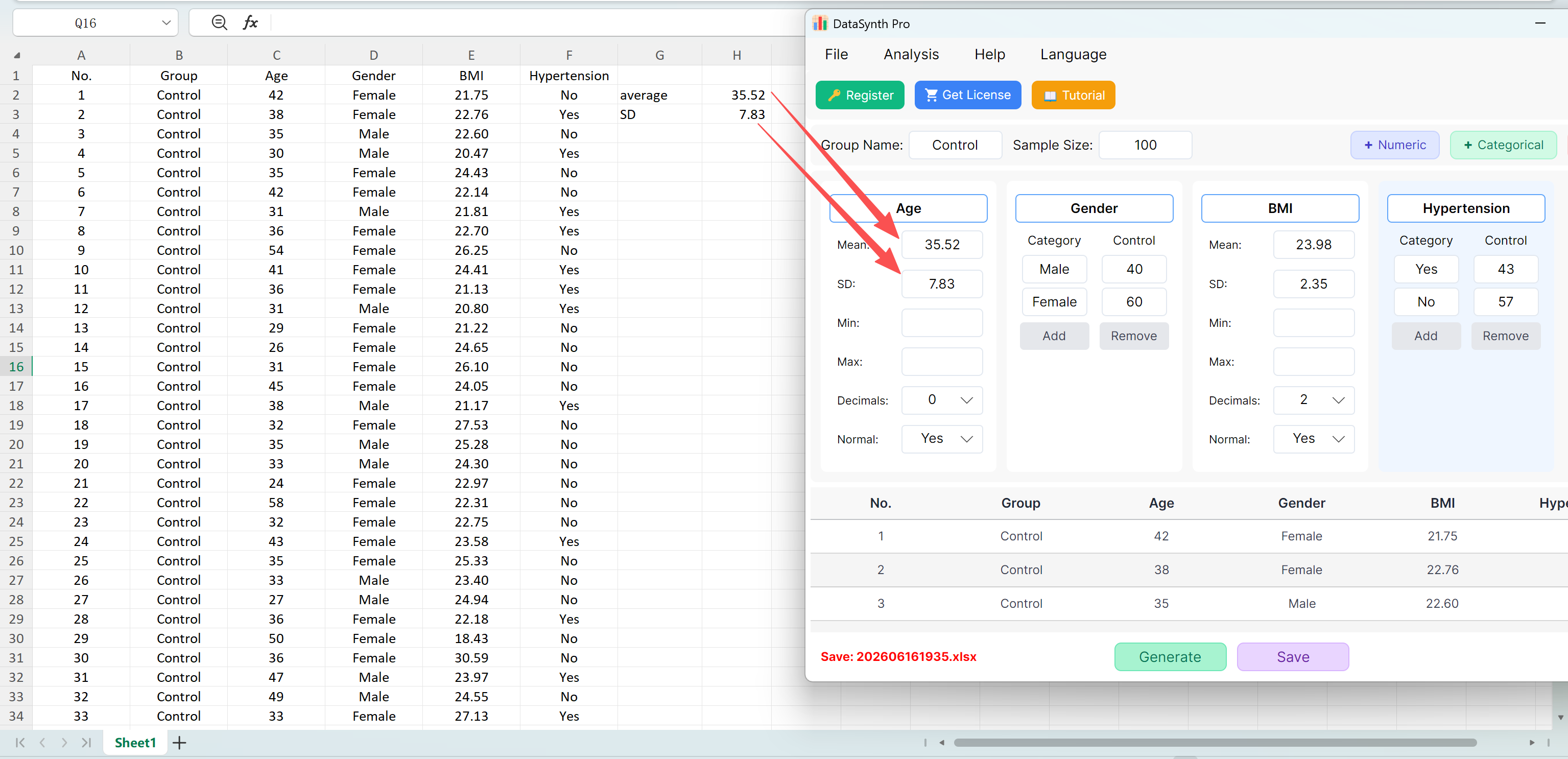
Figure 1.8: Verification Results Identical to Initial Settings
1.6 Computational Efficiency
Equipped with a high-performance optimization engine, the software can generate datasets containing thousands or tens of thousands of records in seconds. If the system fails to converge after maximum iterations, please double-check the statistical plausibility of your configuration, or try running the query without Min/Max limits. The program supports decimal precision of up to 8 places to meet specialized scientific research needs.
Tips & Recommendations:
• Normal Distribution Preference: Data defaults to a normal distribution for seamless downstream analysis (e.g., Independent Samples t-Tests). If you prefer non-parametric or custom-distributed datasets, simply switch the Normal Distribution setting to No.
2. Independent Samples t-Test
Designed for cross-sectional studies comparing the means of two distinct groups. Widely utilized in clinical trials (e.g., drug efficacy between Treatment and Placebo groups) and sociological surveys.
2.1 Workflow
Navigate to Analyze → Independent T-Test. The configuration window will appear as shown below:
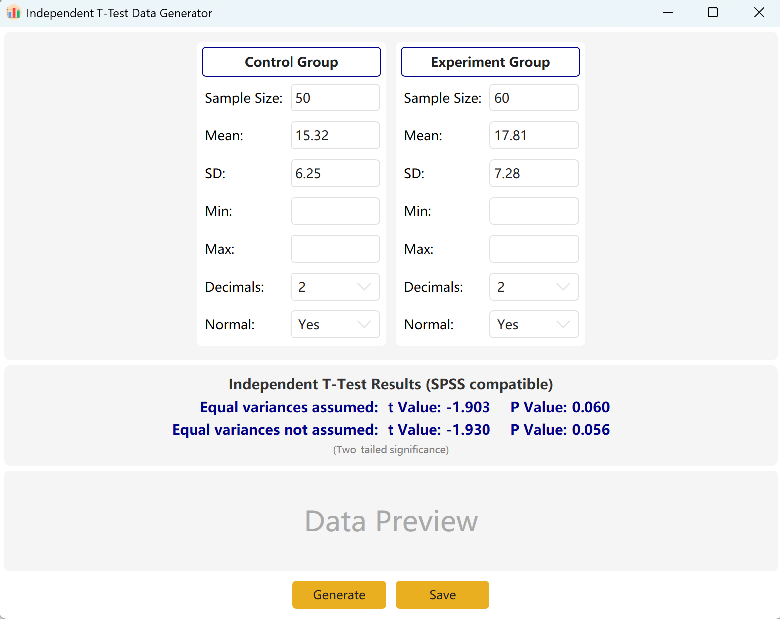
Figure 2.1: User Interface / Operations for Independent T-Test
2.2 Parameters
The program pre-populates sample setups for a 'Control Group' and an 'Experimental Group' as references. Input the Sample Size, Mean, and Standard Deviation for each group to preview the calculated t-value and p-value in real time. Min and Max parameters are optional.
Clicking the Generate Button will create raw datasets for both groups in the preview table below, and the final t-value and p-value will adjust to reflect the actual generated data, using Levene's Test for Equality of Variances.
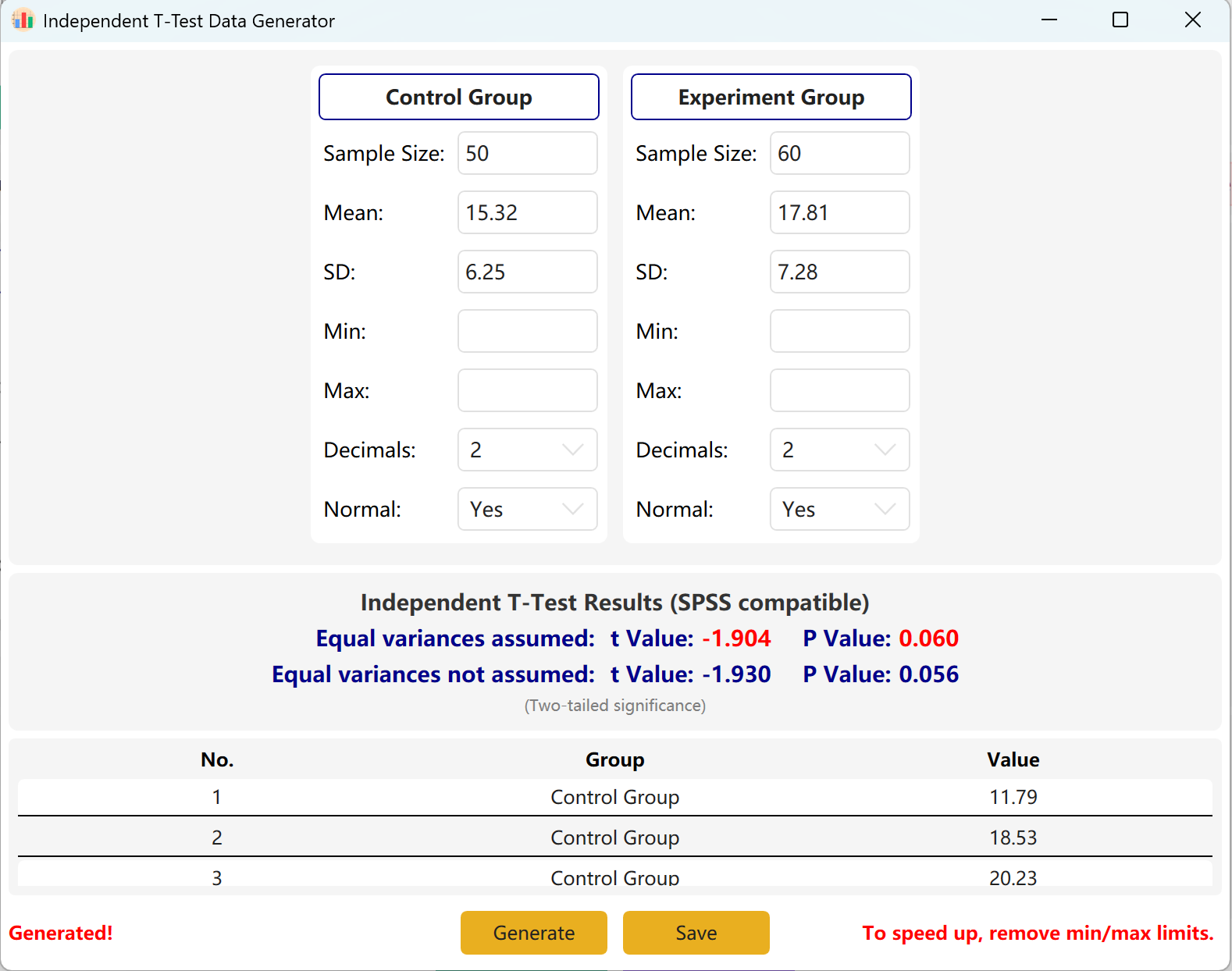
Figure 2.2: User Interface / Operations for Displaying Independent Samples T-Test Data
3. Paired Samples t-Test
Employed for longitudinal or crossover studies where the same subjects are measured twice (e.g., Pre-test vs. Post-test). Focuses on synthesizing the mean difference between paired observations.
3.1 Workflow
Navigate to Analyze → Paired T-Test. The workspace layout is shown below:
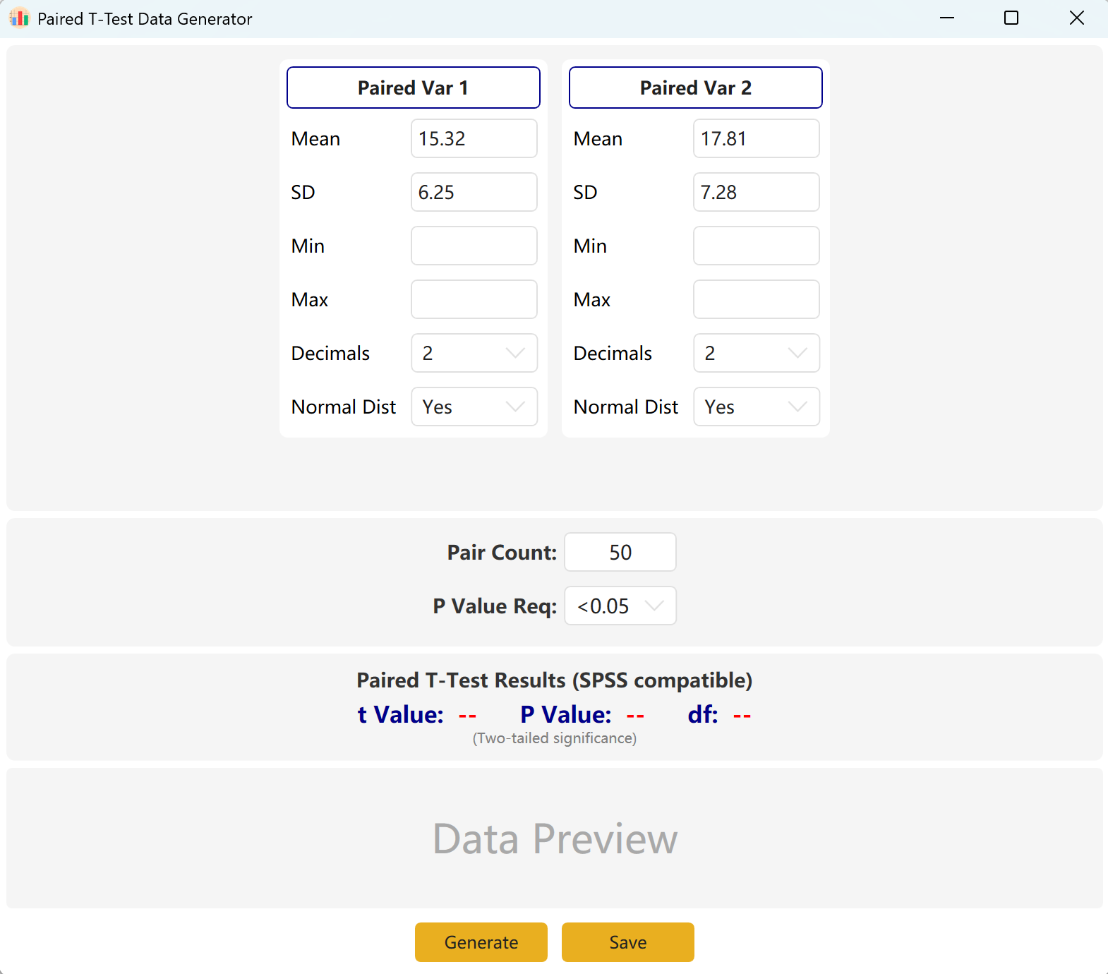
Figure 3.1: User Interface / Operations for Paired T-Test
3.2 Simulation Logic
The software defaults to two paired variables, Paired Var1 and Paired Var2. You can define the Mean and Standard Deviation for each variable, set the overall Sample Size, and establish a target p-value range for the paired t-test. The engine will iteratively compute a compliant dataset.
Convergence Adaptation: If the configured means are mathematically inconsistent with the targeted p-value (e.g., if the two means are highly distinct but you request a non-significant p > 0.05), the program will hold the first group's parameters constant and dynamically adjust the second group's mean to achieve the target p-value.
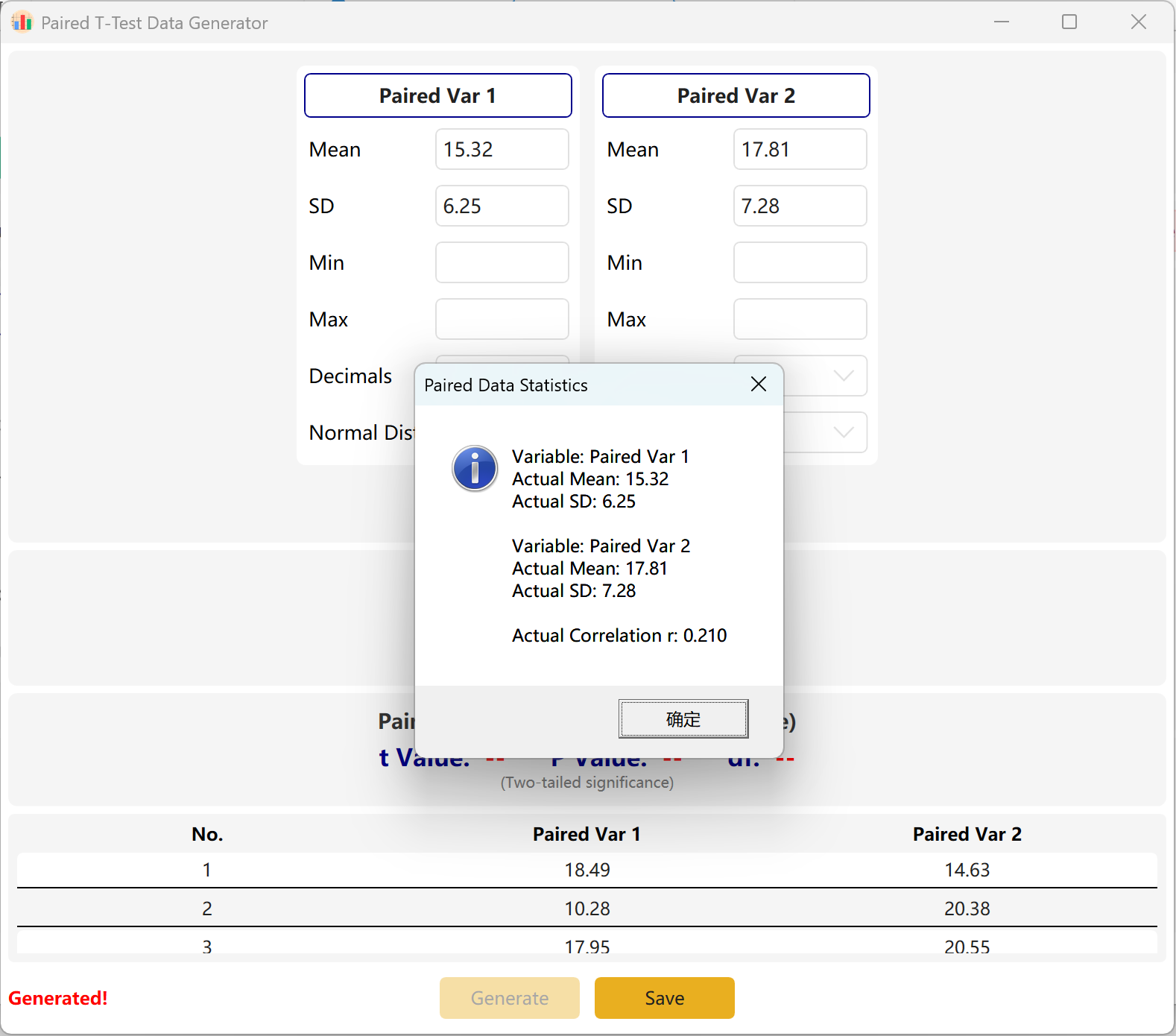
Figure 3.2: User Interface / Operations for Displaying Paired Samples T-Test Data
4. Chi-Square Test
Determines if there is a significant association between two categorical variables. Widely used for demographic cross-tabulations.
4.1 Workflow
Navigate to Analyze → Chi-Square Test. The configuration pane opens as follows:
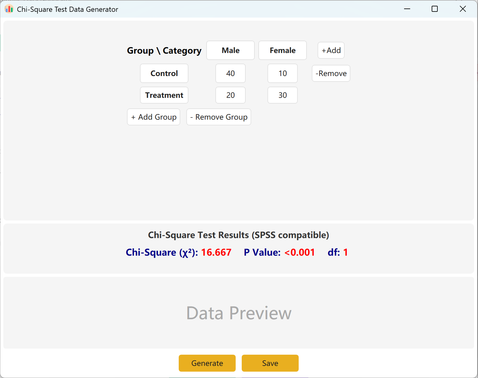
Figure 4.1: User Interface / Operations for Chi-Square Test
4.2 Contingency Matrix
The interface defaults to a standard 2x2 contingency table for Chi-Square calculations, where group and category names are fully editable. Fill in the observed frequencies (counts) for each cell, and the computed Chi-Square value and p-value will update in real time.
You can dynamically add groups (rows) or categories (columns) to accommodate larger models. Click Generate button to produce individual raw records matching these frequencies, and click Save to export the dataset to Excel.
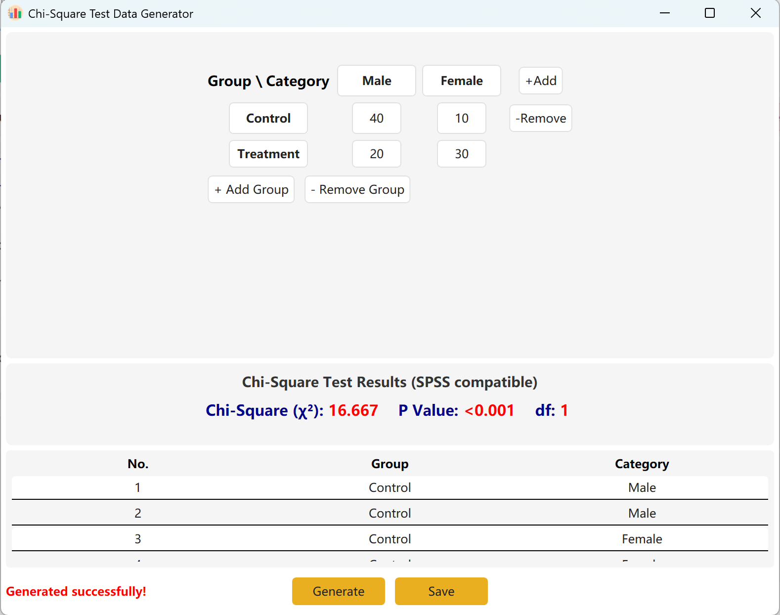
Figure 4.2: User Interface / Operations for Displaying Chi-Square Test Data
5. One-Way ANOVA
Utilized when comparing the means of three or more independent groups. The algorithm synthesizes intra-group variance and inter-group differences to meet target F-values.
5.1 Workflow
Navigate to Analyze → ANOVA → One-Way ANOVA. The workspace layout is as follows:
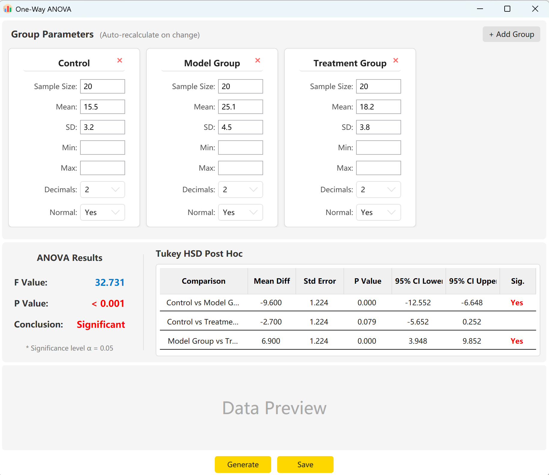
Figure 5.1: User Interface / Operations for One-Way ANOVA
5.2 Configuration
The system pre-loads parameters for three groups: 'Control Group', 'Experimental Group', and 'Treatment Group'. Simply input the Sample Size, Mean, and Standard Deviation for each group to instantly preview the overall F-statistic, p-value, and Tukey's HSD post-hoc multiple comparison results.
Click Generate button to compute and preview raw individual records below. The overall F-value and p-value will automatically update to represent the actual generated values.
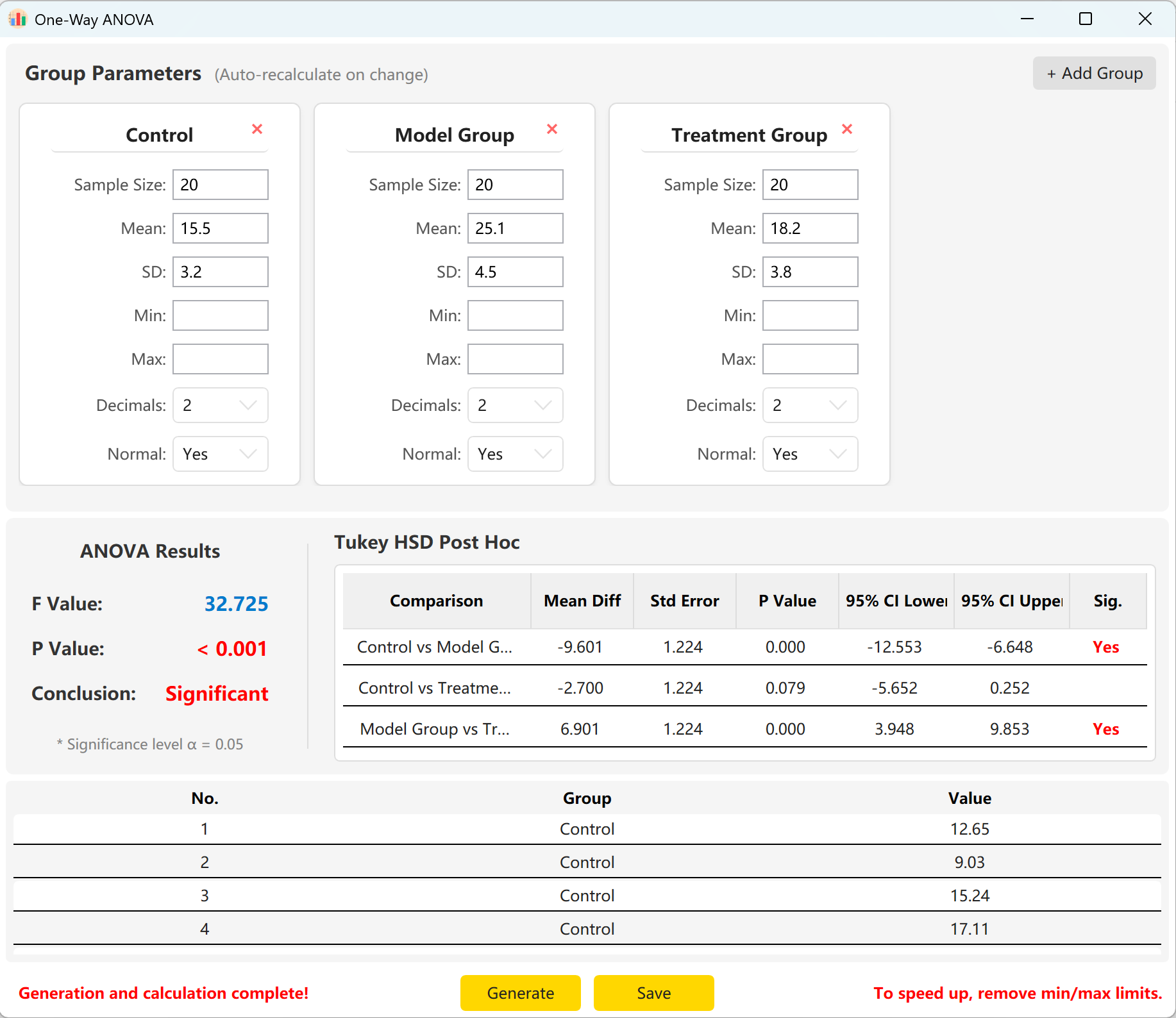
Figure 5.2: User Interface / Operations for Displaying One-Way ANOVA Data
6. Two-Way ANOVA
Examines the influence of two independent categorical variables on one continuous dependent variable. Essential for factorial designs to evaluate main effects and interaction effects.
6.1 Workflow
Navigate to Analyze → ANOVA → Two-Way ANOVA. The configuration pane is displayed below:
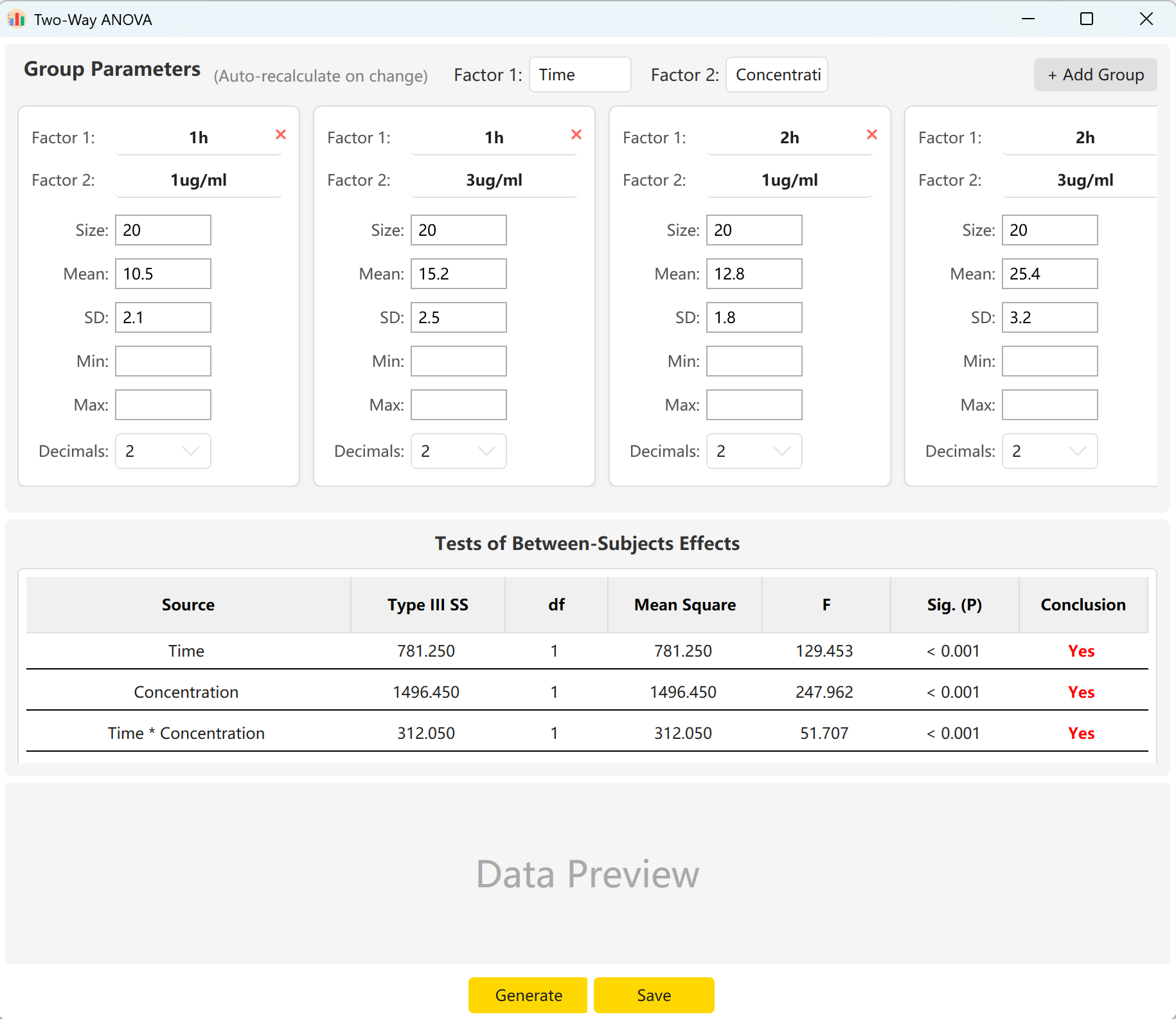
Figure 6.1: User Interface / Operations for Two-Way ANOVA
6.2 Factors & Interactions
The tool defaults to two factors: 'Time' (2 levels) and 'Concentration' (2 levels). Click Add Group to configure more levels if a factor contains multiple classifications.
By filling in the Sample Size, Mean, and Standard Deviation for each cell, you can preview the F-statistics and p-values for the main effect of Time, the main effect of Concentration, and their interaction effect (Time × Concentration). Click Generate button to construct the matching individual raw records in the preview pane.
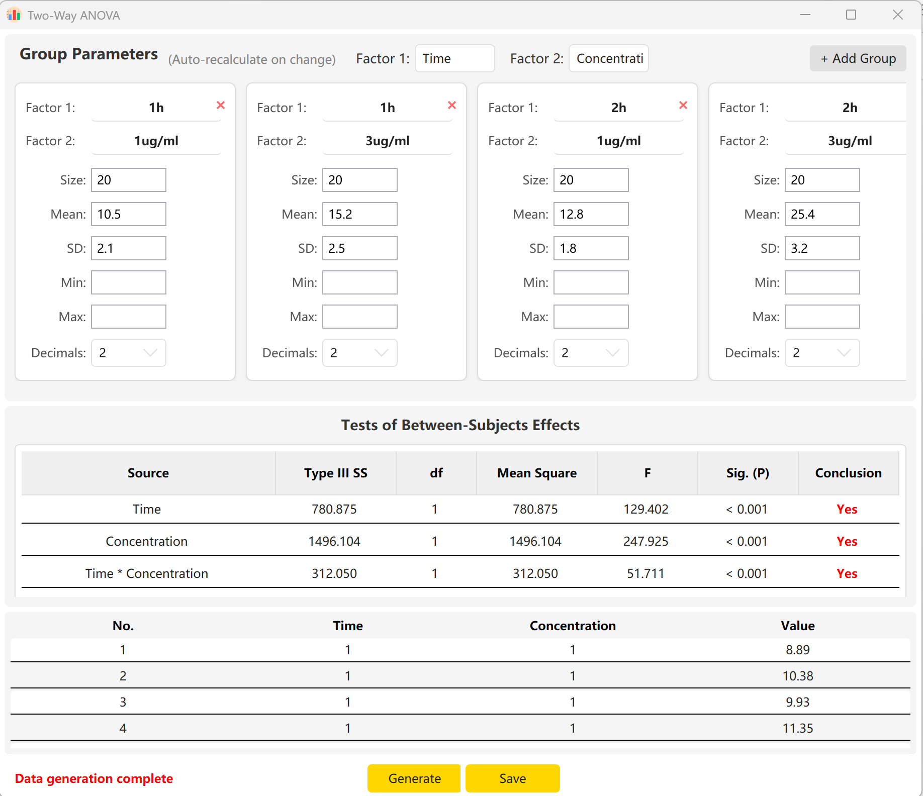
Figure 6.2: User Interface / Operations for Displaying Two-Way ANOVA Data
7. One-Way Repeated Measures ANOVA
The extension of Paired T-Test to three or more time points. Ideal for longitudinal tracking over extended periods (e.g., baseline, month 1, month 3).
7.1 Workflow
Navigate to Analyze → ANOVA → Repeated Measures ANOVA. The workspace layout is shown below:
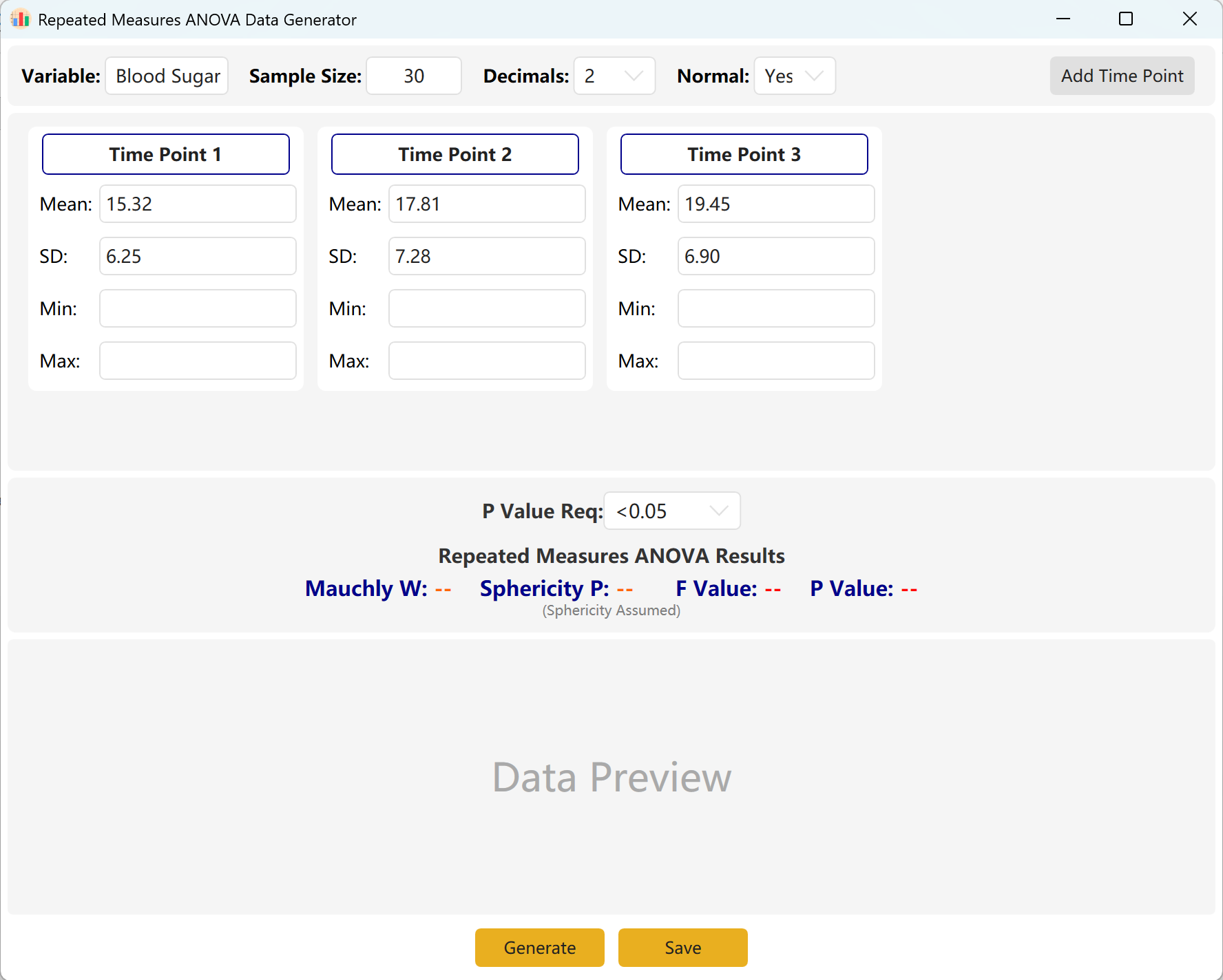
Figure 7.1: User Interface / Operations for One-Way Repeated Measures ANOVA
7.2 Repeated Observations
The system defaults to three observation time points. You can easily scale this up by clicking the Add Time Point button. Input the Mean and Standard Deviation for each time point and define your target p-value range.
Click Generate button to synthesize compliant values.
Engine Compression: If the difference between time points is mathematically massive (indicating a highly significant p-value) but your target range is set to p > 0.05, the engine will automatically compress the variances and mean differences among time points to meet your exact target p-value. A pop-up dialog will present the actual statistics of the synthesized dataset.
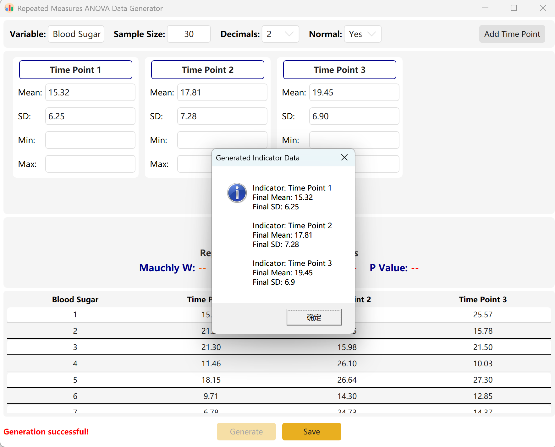
Figure 7.2: User Interface / Operations for Displaying Repeated Measures ANOVA Data
8. Two Independent Samples Rank Sum Test (Non-parametric)
Mann-Whitney U test alternative for data that fails normality assumptions. Evaluates median differences based on rank-order logic on continuous or ordinal variables.
8.1 Workflow
Navigate to Analyze → Non-parametric → 2 Independent Samples. The configuration workspace is shown below:
1.png)
Figure 8.1: User Interface / Operations for Two Independent Samples Rank Sum Test
8.2 Setup
The program defaults to two reference groups. Since non-parametric methods are designed for non-normally distributed data, the Normal Distribution option is set to No by default. Using the Mann-Whitney U Test, you can define a target p-value range. Click Generate button to synthesize raw observations that statistically comply with this threshold.
Rank Sum Generation Logic: Non-parametric tests analyze group differences by pooling all observations and assigning ranks. Therefore, if the configured parameters of the two groups are highly distinct (naturally yielding a very small p-value) but you set a target threshold of p > 0.05, the engine will automatically reduce the divergence between groups to satisfy your target. The final calculated means and standard deviations will be displayed in a pop-up dialog.
2.png)
Figure 8.2: User Interface / Operations for Displaying Two Independent Samples Rank Sum Test Data
9. Kruskal-Wallis Test (K Independent Samples Non-parametric)
Kruskal-Wallis H test equivalent. Generates ordinal or non-normally distributed continuous data across three or more independent groups.
9.1 Workflow
Navigate to Analyze → Non-parametric → K Independent Samples. The configuration workspace is shown below:
1.png)
Figure 9.1: User Interface / Operations for Kruskal-Wallis Test
9.2 Multi-Group Ranking
The program defaults to three reference groups and performs a Kruskal-Wallis Test. Just like the two-group test, because calculations are rank-based on a pooled dataset, if the configured multi-group parameters have massive discrepancies (yielding highly significant p-values) but you request a target of p > 0.05, the simulation engine will automatically compress the inter-group differences. The resulting statistics will be summarized in a pop-up window.
2.png)
Figure 9.2: User Interface / Operations for Displaying Kruskal-Wallis Test Data
10. Quartile Data Generation
Divides a rank-ordered dataset into four equal parts. Useful for evaluating the spread and central tendency of data, highlighting the median, and detecting outliers.
10.1 Workflow
Navigate to Analyze → Quartile Data. The layout is illustrated below:
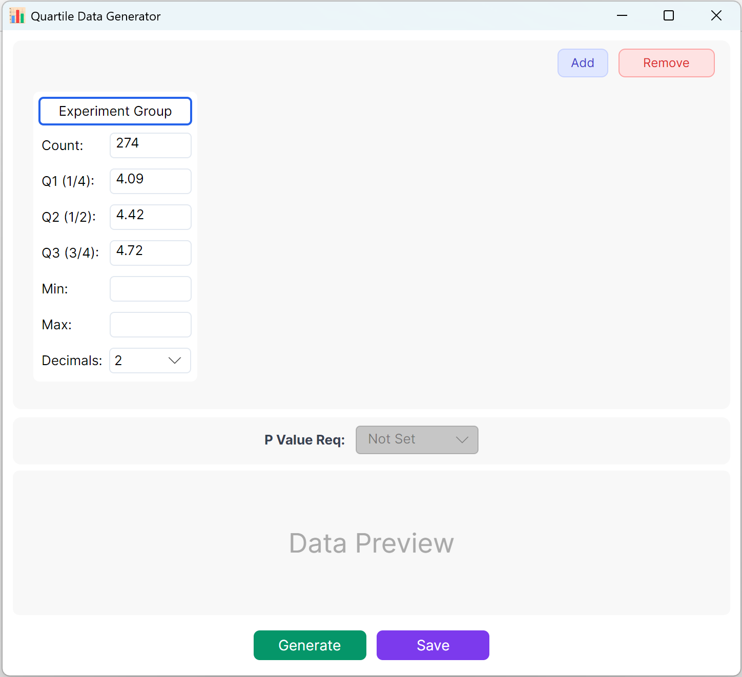
Figure 10.1: User Interface / Operations for Quartile Data
10.2 Parameter Definition
Define your targeted Sample Size, Q1 (25th percentile), Q2 (Median / 50th percentile), and Q3 (75th percentile). Min/Max boundaries can be left blank if there are no specific constraints. Choose your decimal precision and click Generate button to produce observations meeting these exact quartile boundaries.
Summary: Configure sample sizes and target values for Q1, Q2, and Q3. Optional parameters include Minimum, Maximum, and Decimal Places. Click Generate button to compute and display raw observations matching the targeted quartile structure. For multi-group setups, you may also lock in a targeted inter-group p-value range.
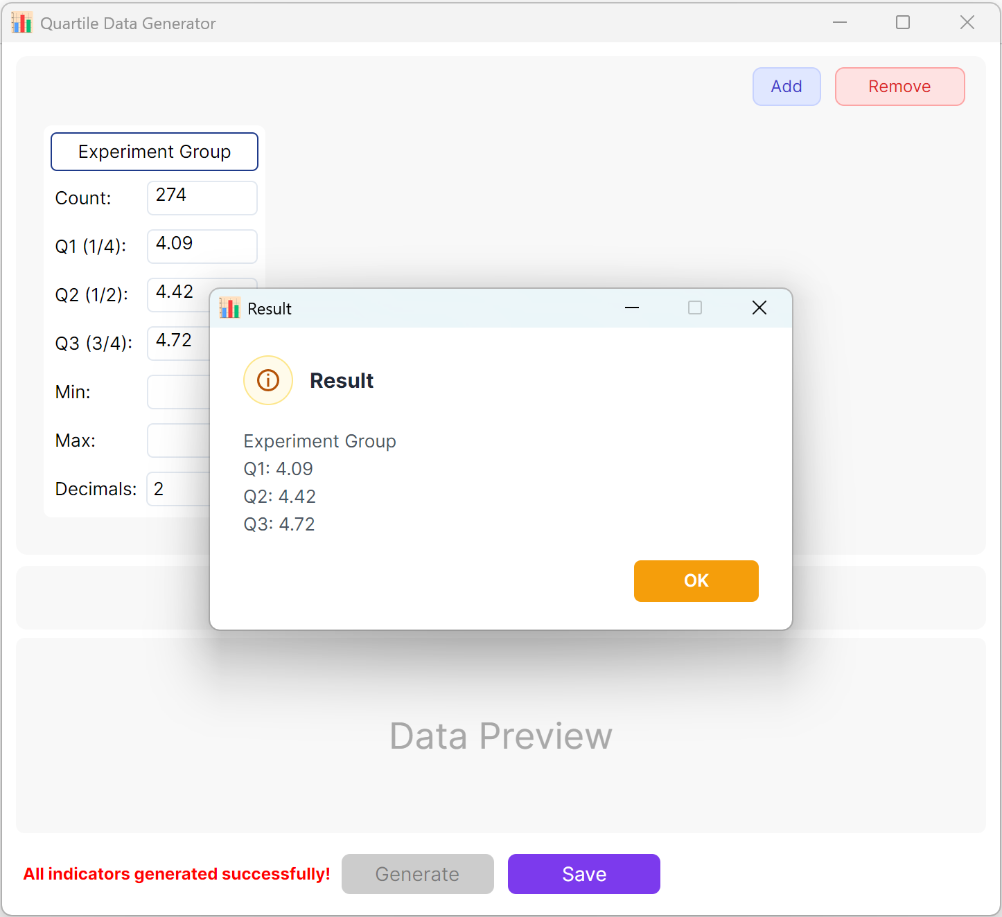
Figure 10.2: User Interface / Operations for Displaying Quartile Data
11. Binary Logistic Regression Data Generation
Essential for classification problems where the outcome is dichotomous (DV=0 or DV=1). Highly prevalent in epidemiology for risk factor identification (e.g., Disease vs. Healthy).
11.1 Workflow
Navigate to Analyze → Regression → Binary Logistic.
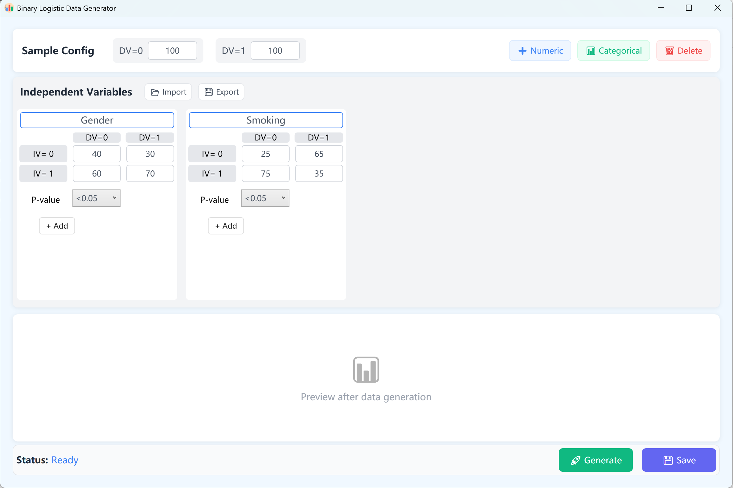
Figure 11.1: User Interface / Operations for Binary Logistic Regression
11.2 Design
By default, two continuous independent variables are set up as references. In a binary logistic model, the dependent variable has exactly two outcomes (0 and 1). Accordingly, the dependent variable is structured as 0 and 1 groups, defaulting to a sample size of 100 cases per category (which can be customized).
- Variable Setup: Click + Numeric to add continuous independent variables (e.g., 'Age', 'BMI'). Enter the Variable Name, Mean, Standard Deviation, Decimal Places, and target p-value range (this specifies the target significance level you want the variable to achieve in the final logistic regression model). Min/Max constraints are optional.
- Generation & Validation: Click Generate button to run the synthesis algorithm. The system will iteratively compute a dataset where the logistic regression model yields p-values matching your configuration.
A detailed Regression Analysis Report matching IBM SPSS formatting will automatically pop up. Closing this report displays the raw dataset in the preview table, ready to be exported to Excel.
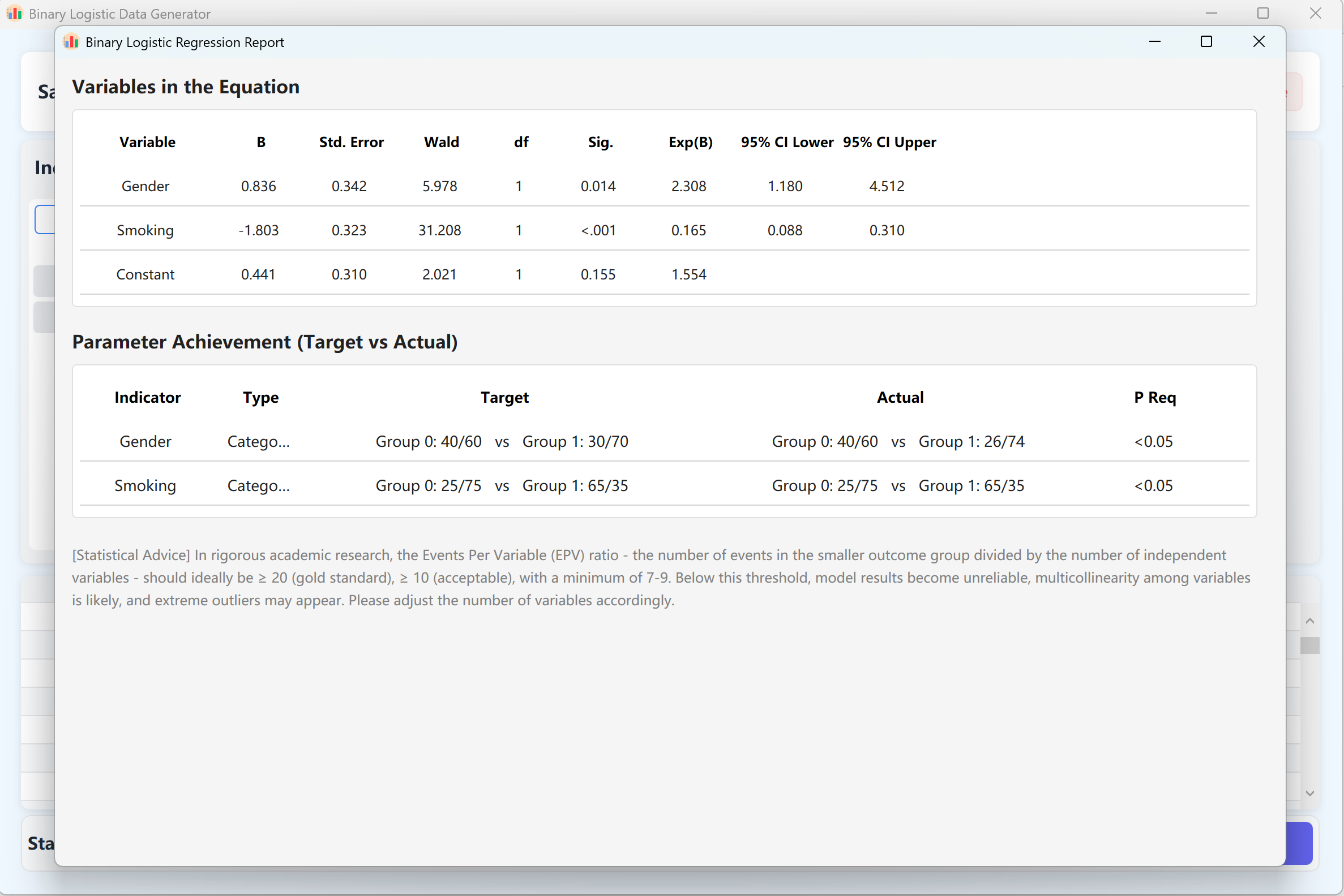
Figure 11.2: User Interface / Operations for Displaying Binary Logistic Regression Data
12. Multiple Linear Regression Data Generation
A core predictive modeling tool. It synthesizes a continuous Dependent Variable (Y) influenced by multiple Independent Variables (X), which can be continuous numerical, quartiles, ordered categorical (ordinal), or unordered categorical (nominal).
12.1 Workflow
Navigate to Analyze → Regression → Linear Regression.
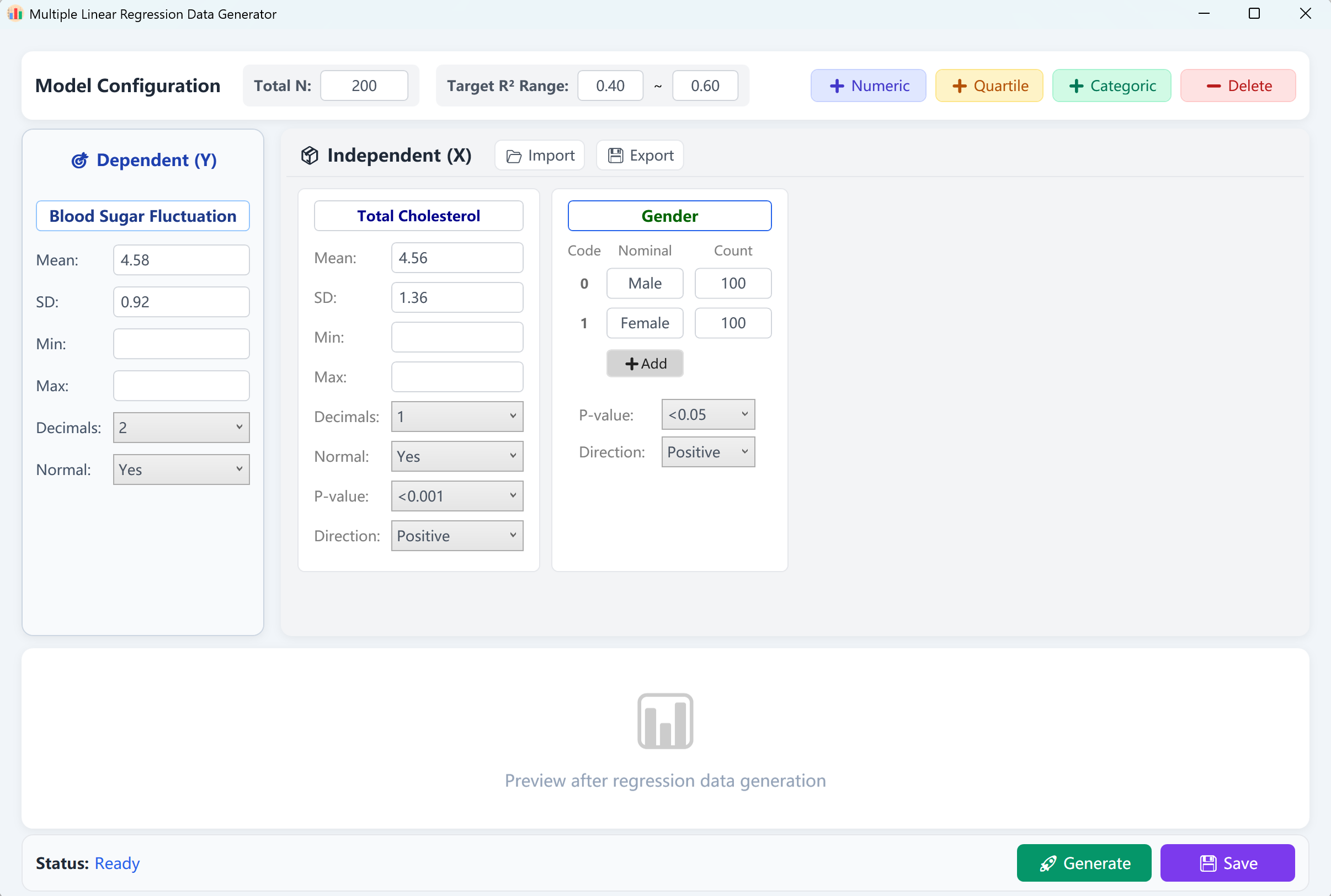
Figure 12.1: User Interface / Operations for Multiple Linear Regression
12.2 Model Settings
The interface pre-loads a continuous dependent variable ('Blood Glucose Fluctuation') and two independent variables ('Total Cholesterol' as numerical, 'Gender' as categorical) with a default sample size of 200 cases. You can configure a target R-squared (R²) range (e.g., 0.4 to 0.6).
Click Generate button to run the regression model. A validation report matching SPSS output will pop up. Closing this report returns you to the raw data preview table, which can be saved as an Excel spreadsheet.
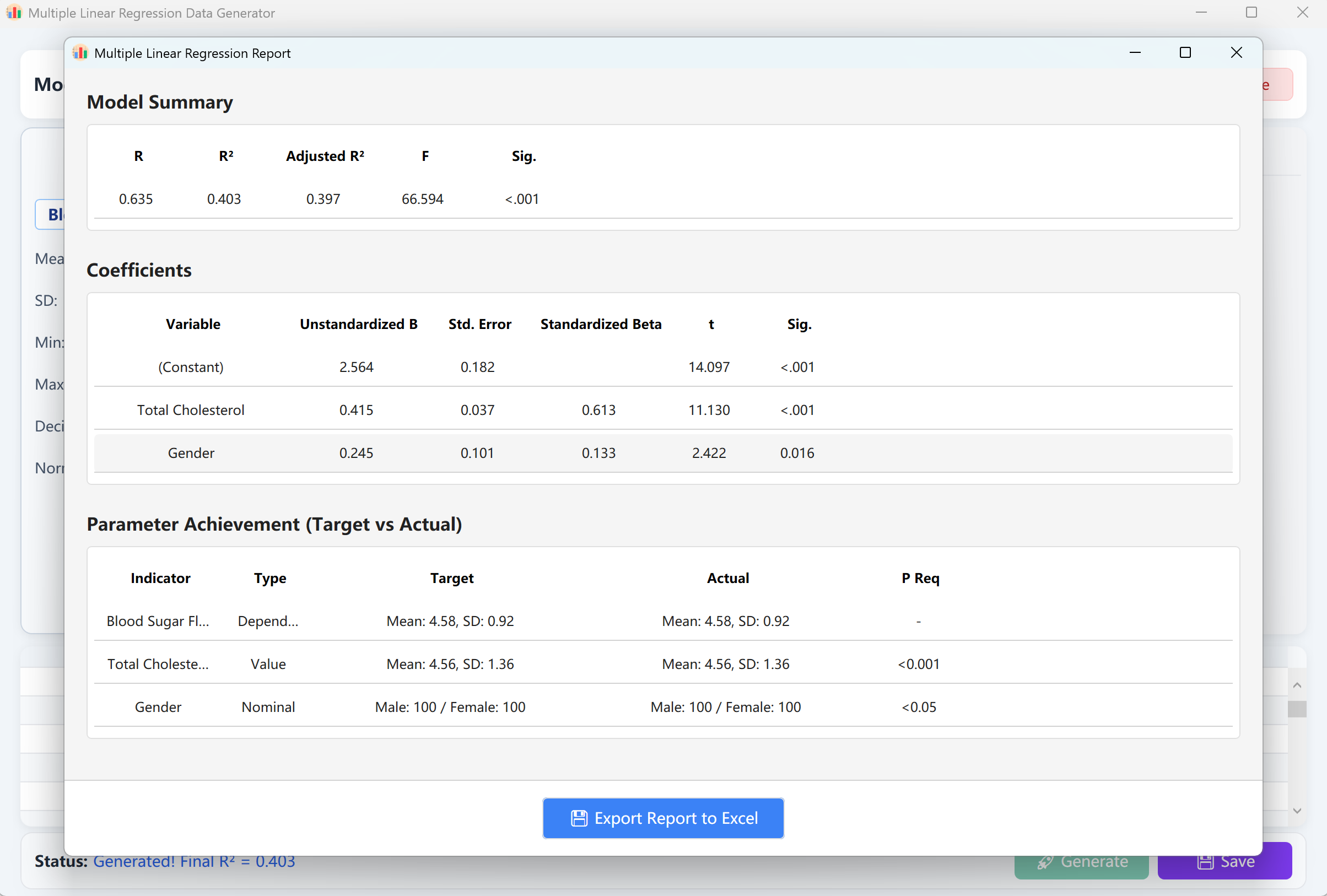
Figure 12.2: User Interface / Operations for Displaying Multiple Linear Regression Data
13. Cox Proportional Hazards Regression Data Generation
The gold standard for survival analysis. Simulates time-to-event data while accounting for right-censoring, allowing researchers to evaluate the effect of covariates on survival times.
13.1 Workflow & Technical Guidelines
Navigate to Analyze → Regression → Cox Regression.
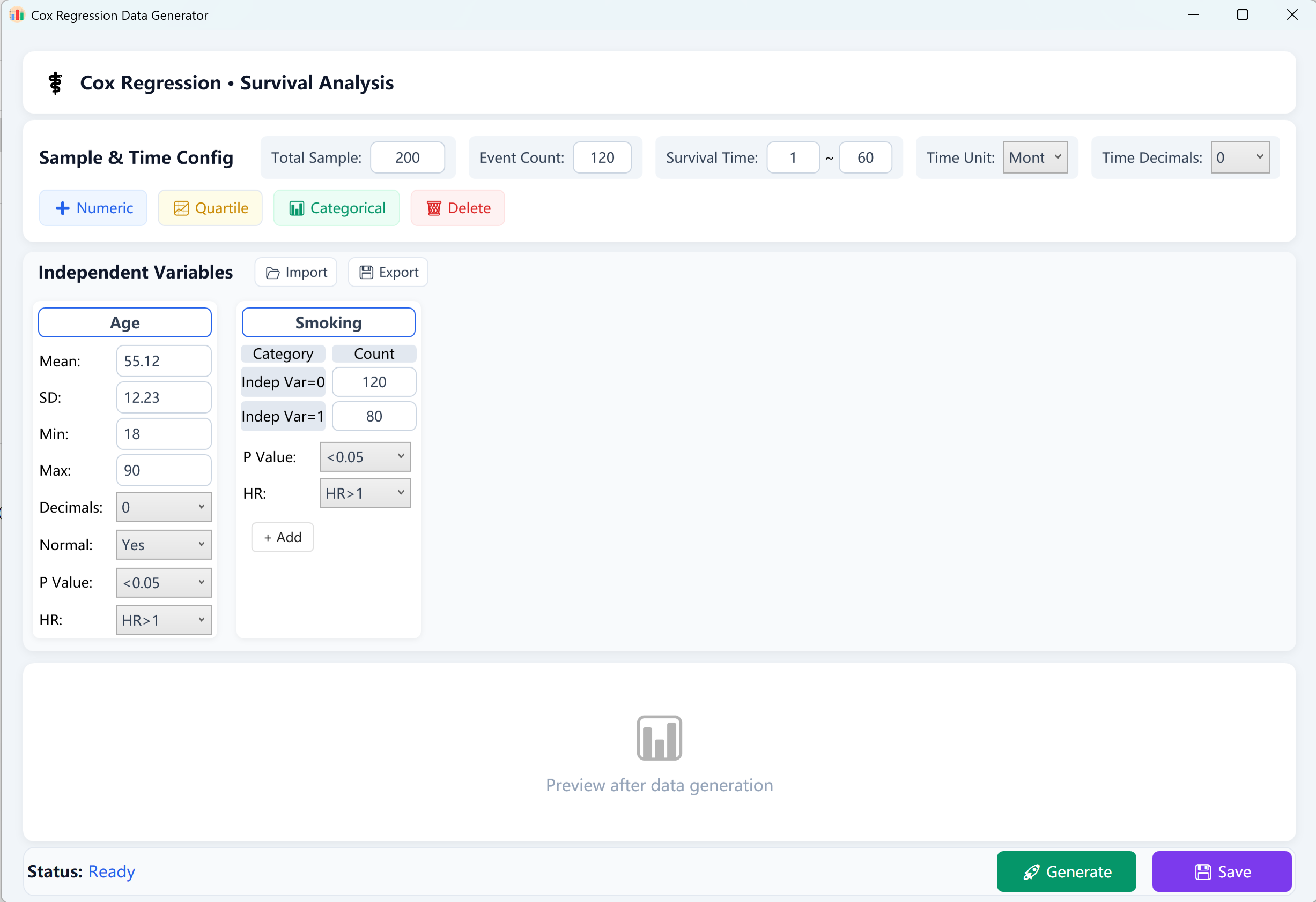
Figure 13.1: User Interface / Operations for Cox Proportional Hazards Regression
- Total Sample Size (N): The overall number of subjects/patients (e.g., 200 subjects).
- Observed Events (Outcome Events): The count of positive cases that experienced the terminal outcome (e.g., death, recurrence, or event failure) during the follow-up period. Note: The number of events must be strictly less than the total sample size.
- Survival Time Range (T): Define [Min Follow-up] to [Max Follow-up] bounds of survival duration (e.g., 1~60 months), label time in days, months, or years, and define the numerical decimal precision.
Statistical EPV Rule (Events Per Variable): To guarantee the mathematical stability and reliability of a Cox Proportional Hazards model, it is highly recommended that the ratio of observed outcome events to the number of independent variables (EPV) is at least 10 to 20. If your model fails to converge, try increasing either the overall Sample Size or the number of Observed Events.
13.2 Constructing Research Variables
Click corresponding buttons at the bottom of the variable card to construct independent covariates:
- Continuous Numerical Variables: Click + Numeric to add continuous covariates (e.g., Age, BMI, clinical biomarkers). Fill in Mean, Standard Deviation (required), and optionally Min/Max boundaries to restrict outlier bounds and decimal precision.
- Categorical Variables: Click + Categorical to add nominal/ordinal covariates (e.g., Gender, Satisfaction Score). Input the exact target frequency for each category. Note: The sum of counts across all categories must strictly equal the Total Sample Size to run.
- Quartile Variables: Click + Quartile to add quartile-structured variables, filling in Q1, Q2 (Median), and Q3 target parameters.
Target Parameters: Every variable card contains two powerful target parameters at the bottom:
- Regression p-value: Choose significance targets (e.g., p > 0.05, p < 0.05, p < 0.01, or p < 0.001).
- Hazard Ratio (HR) Direction: Choose either HR > 1 (a risk factor, indicating increased hazard rate) or HR < 1 (a protective factor, indicating reduced hazard rate).
13.3 Executing Data Generation and Saving
Once all parameters are filled, click Generate button at the bottom of the window. The backend will execute highly concurrent iterative simulations. An authoritative and comprehensive Cox Proportional Hazards Regression Analysis Report will automatically pop up, mirroring the exact statistics and styling calculated by IBM SPSS.
Click Save button to export the synthesized raw dataset into an Excel file, which can easily be imported into SPSS or other professional statistical suites for verification.
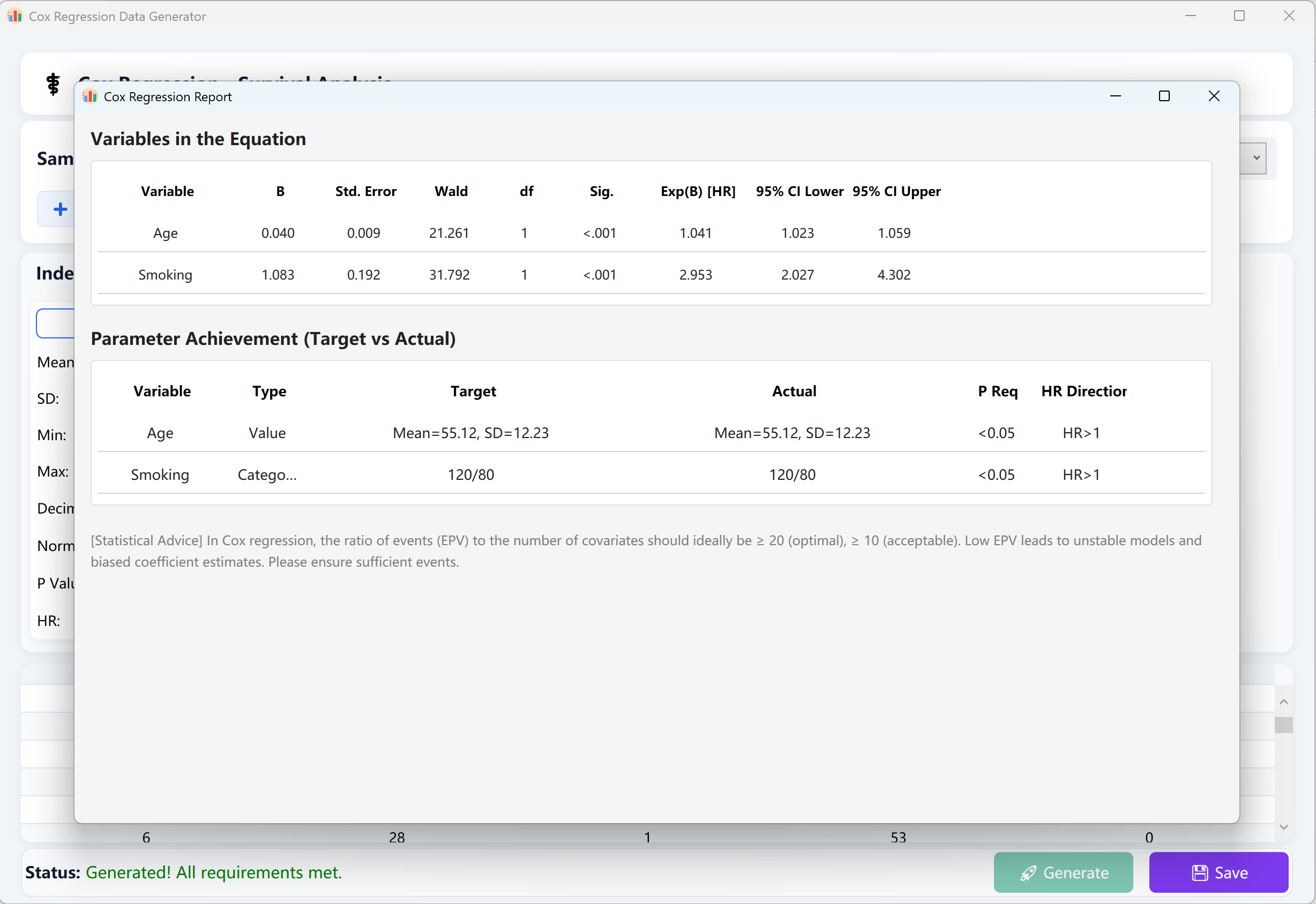
Figure 13.2: User Interface / Operations for Displaying Cox Proportional Hazards Regression Data
14. Generating Data for Correlation Analysis
Simulates bivariate relationships (Pearson or Spearman) and Partial Correlation by enforcing target correlation coefficients (r-values) and significance levels.
14.1 Workflow
Navigate to Analyze → Correlation.
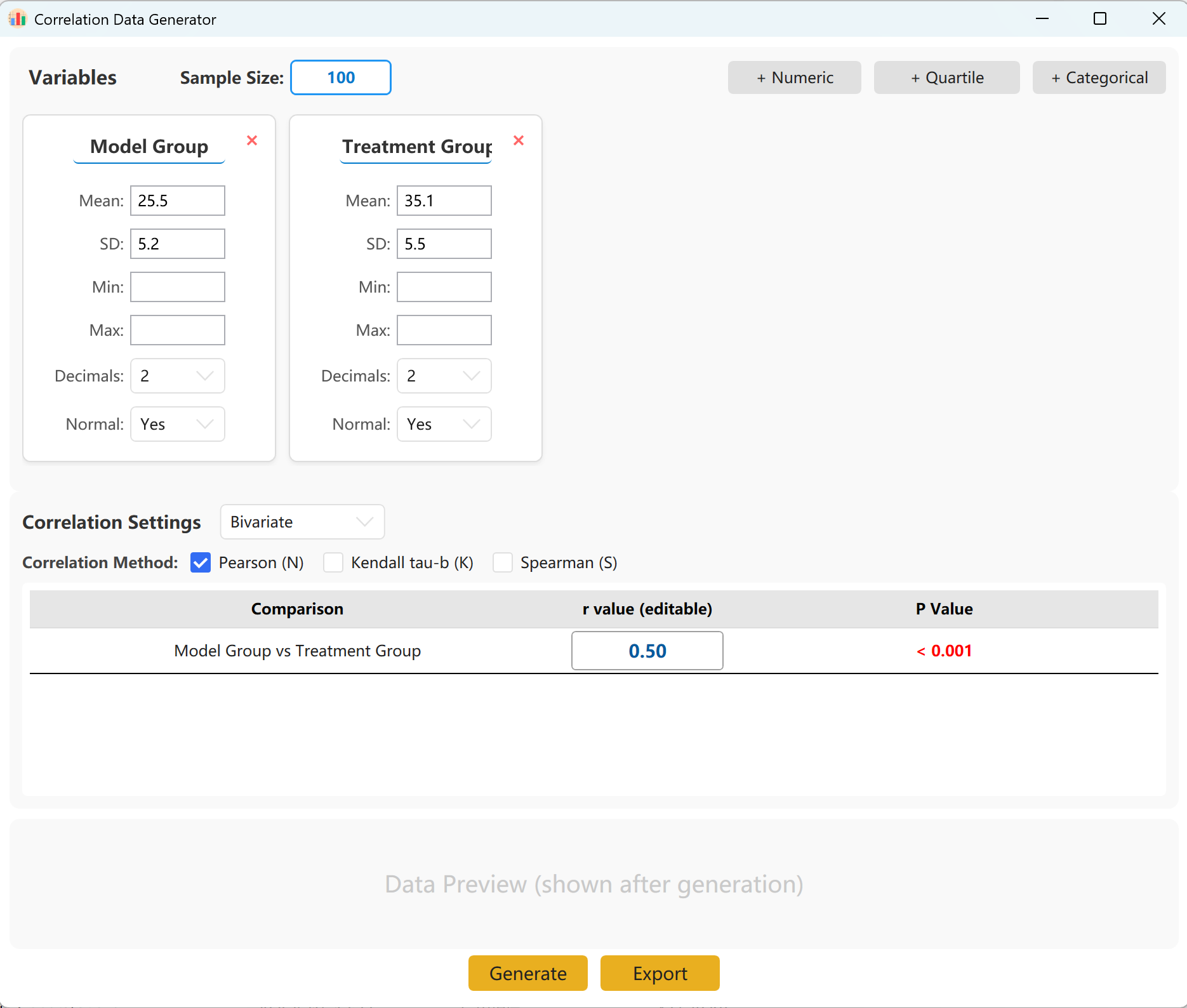
Figure 14.1: User Interface / Operations for Correlation Analysis
14.2 Parameters
The system pre-loads two variable sets for quick reference. You can easily add more variables, supporting continuous (mean/SD), quartile, and categorical forms. Within the configuration panel, specify the Sample Size, Mean, and Standard Deviation for each metric (Min/Max limits are optional).
You can specify the exact target correlation coefficient (r) between groups. Clicking Generate button to run the simulation and display the resulting correlation matrix in a pop-up window, which can then be exported as an Excel file.
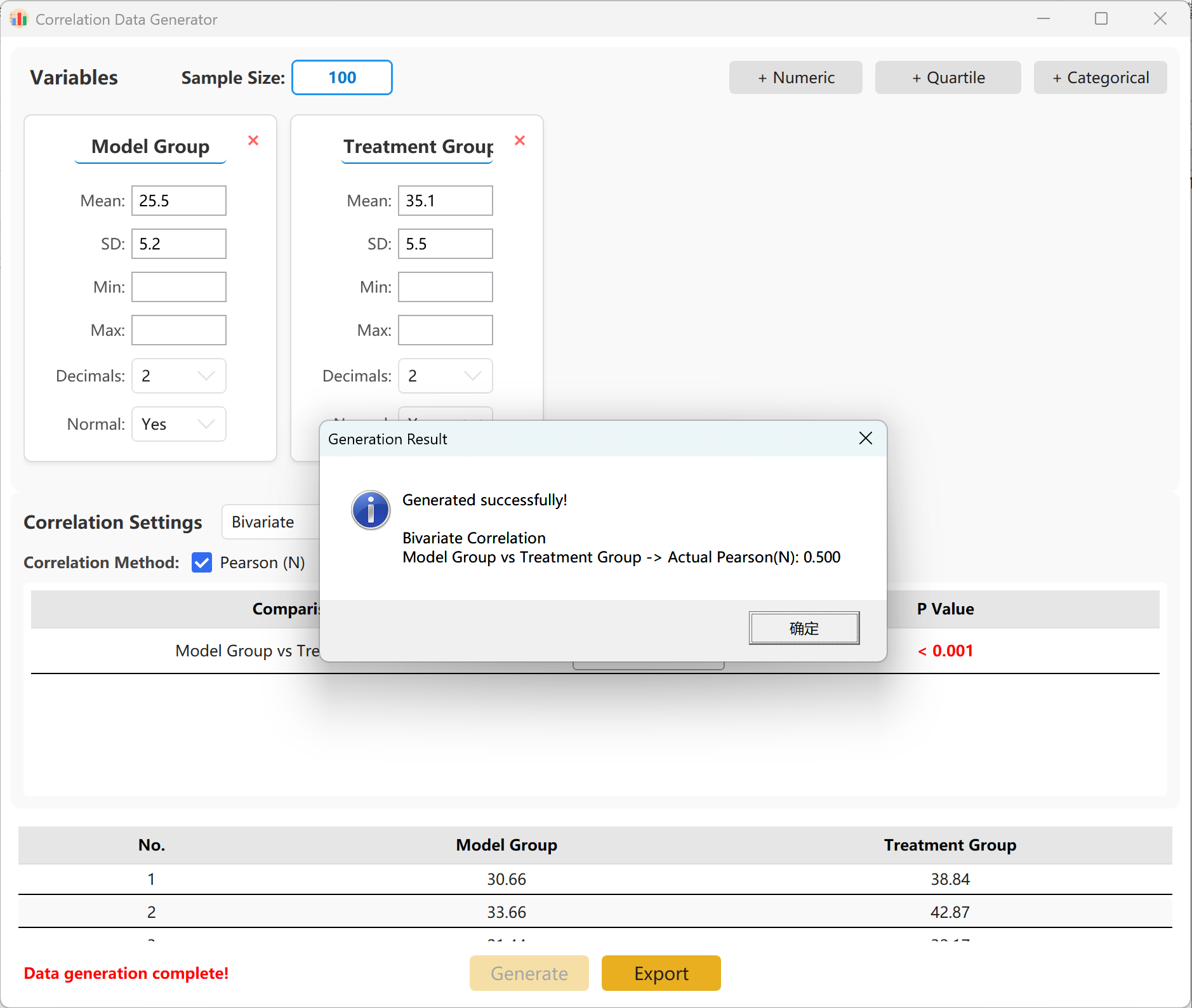
Figure 14.2: User Interface / Operations for Displaying Correlation Analysis Data
15. Generating Data for ROC Curve Analysis
Evaluates the diagnostic ability of a continuous or categorical test variable in distinguishing between two states (e.g., Positive vs. Negative diagnosis).
15.1 Workflow
Navigate to Analyze → ROC Curve.
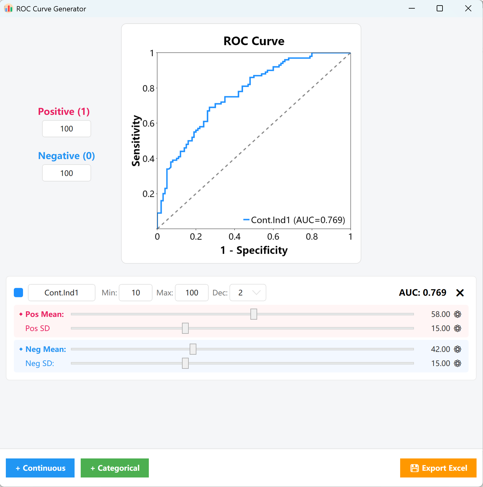
Figure 15.1: User Interface / Operations for ROC Curve Settings
Proportions: In the parameters panel on the left, enter your targeted case counts for Positive Samples (1) and Negative Samples (0) (e.g., 100 positive cases and 100 negative cases). The generation engine will construct the core statistical sampling matrix based on these proportions.
15.2 Variable Types
Click + Continuous or + Categorical at the bottom-left to create corresponding variables:
- Continuous Variables: Customize the Variable Name, Min/Max bounds, and targeted Decimal Places on the card. Drag the Pink slider (Positive group) and Blue slider (Negative group) to rapidly adjust their respective Mean and SD distributions.
- ⚙ Precision Tuning: If the visual sliders cannot reach the exact granularity you need, click the Gear icon (⚙) next to the parameter to manually key in precise floating-point values.
- Monitor AUC: Throughout this tuning process, the AUC = 0.XXX indicator at the top-right of the card and the central plotting canvas will update completely in real time, allowing you to visually align the curve to your exact target cut-off.
- Categorical Variables: Simply define the exact proportions or counts for both positive and negative cohorts. You can immediately monitor the corresponding changes in the ROC curve and the AUC value.
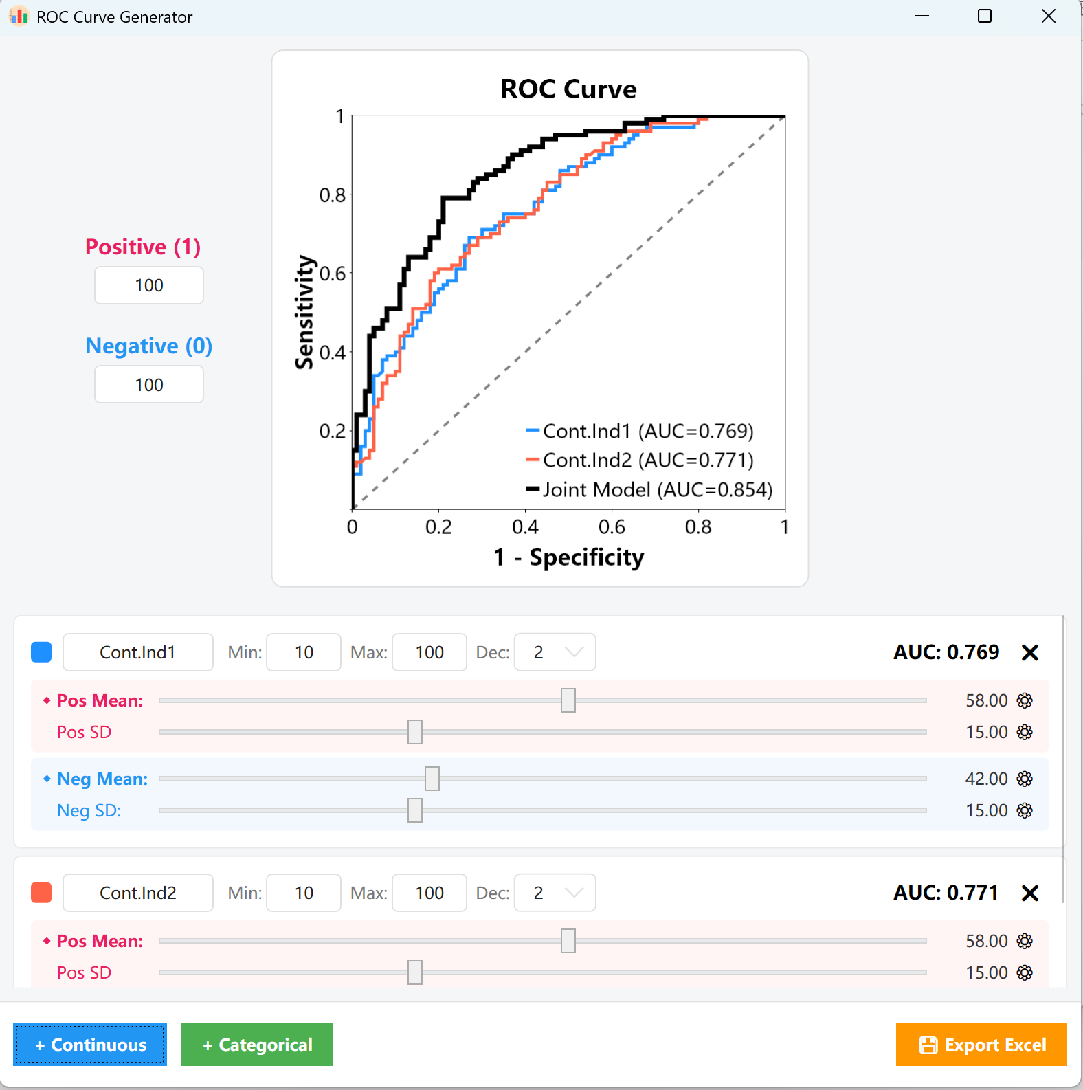
Figure 15.2: User Interface / Operations for Displaying ROC Curve Plot
16. Saving and Exporting Configured Parameters
To streamline repetitive modeling tasks and avoid manual configuration errors, the application provides a powerful built-in configuration state preservation mechanism.
16.1 Save/Restore
- Export Configuration: Navigate to File → Export Configuration to save all configured parameters, variable definitions, group structures, and targets as a local `.json` configuration file on your computer.
- Import Configuration: To restore your setup during a future session, simply navigate to File → Import Configuration and select your previously saved configuration file. The workspace will immediately reload and recover all variable cards, sliders, and parameter values.